Pivot tables are an efficient way to drill down into the details of specific topics while browsing all topics. We’ll walk through how to create and use pivot tables to speed up your content workflow.
1. Go to the Topic Table Tab
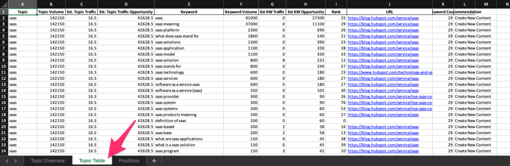
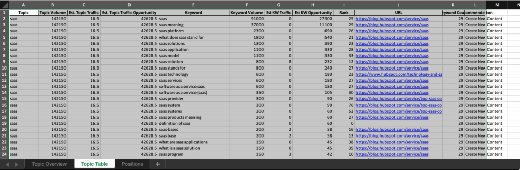
2. Select All Data
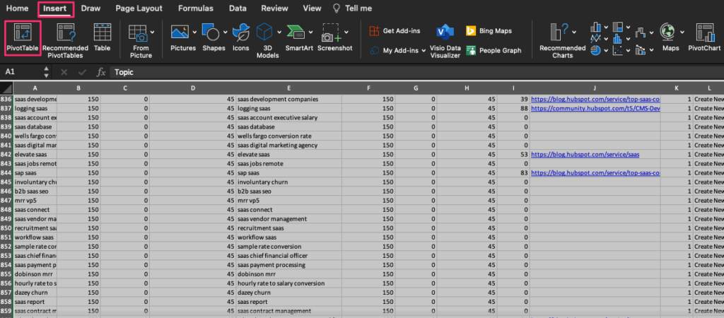
3. Insert Pivot Table
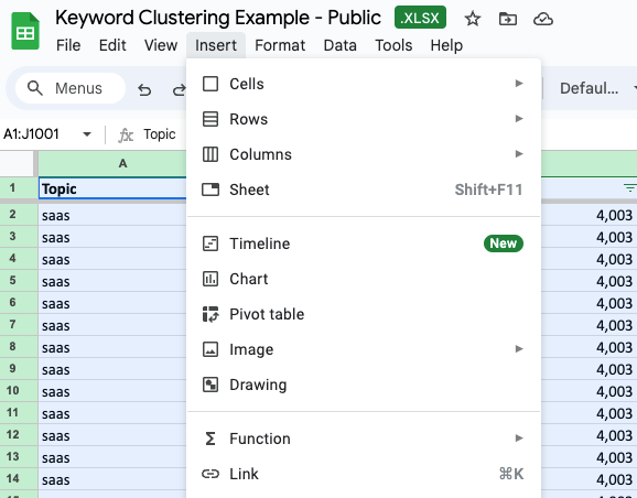
In both Microsoft Excel and Google Sheets, click on the “insert” menu and then “Pivot Table”.
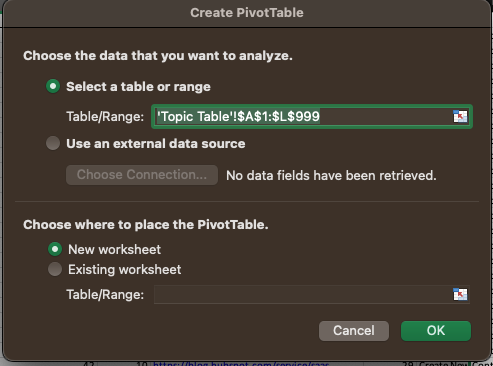
Microsoft Excel
Then verify the range is correct and choose to insert the pivot table into a new worksheet.
Google Sheets
4. Setup Your Pivot Table
Microsoft Excel
A good starting point is to setup your Rows with the Topic first and then Keyword. For the Values, select:
- Sum of Keyword Volume
- Sum of Est KW Traffic
- Sum of Est KW Opportunity
Note, since a pivot table automatically sums your values, you want to make sure you’re dragging the keyword level data in, not the topic level data.
Your pivot table should now look like this with Topics and keywords nested under them:
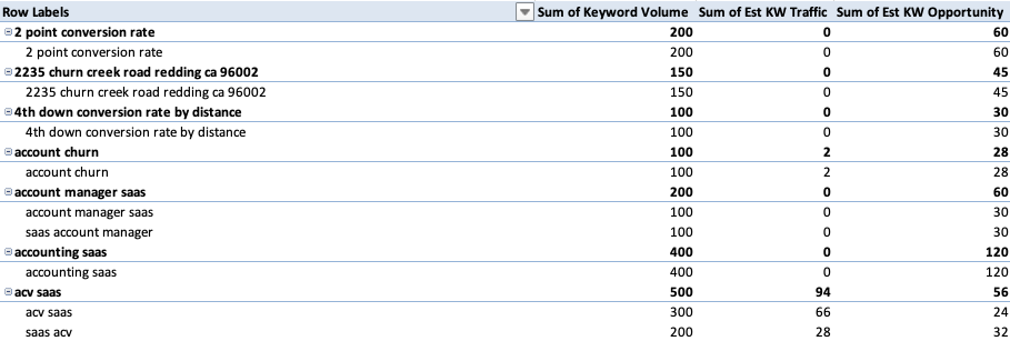
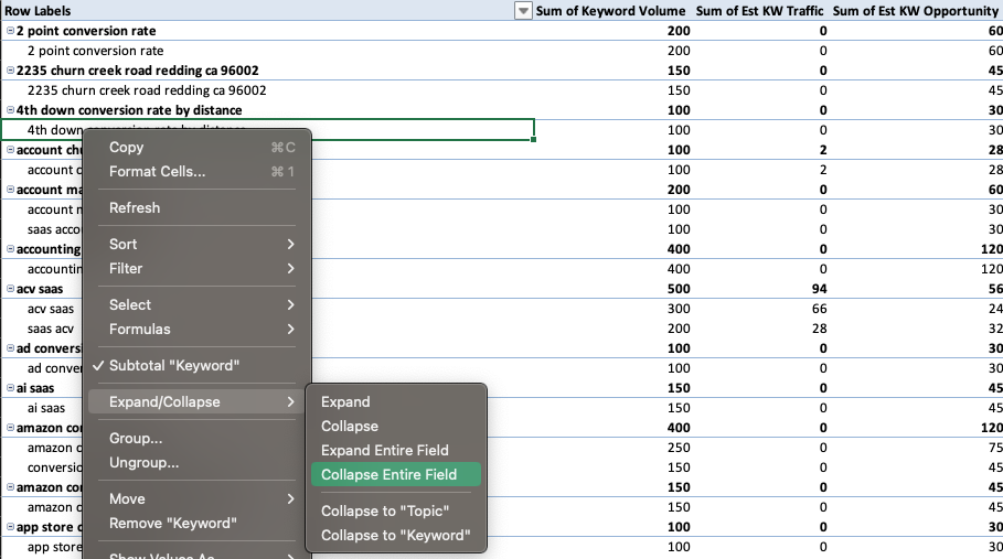
You can collapse all the keywords into their parent topics by right clicking in the pivot table, then going down to “Expand/Collapse” and selecting “Collapse Entire Field”.
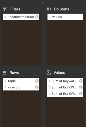
Google Sheets
In Google Sheets, you’ll do the same steps, it just looks a little different:
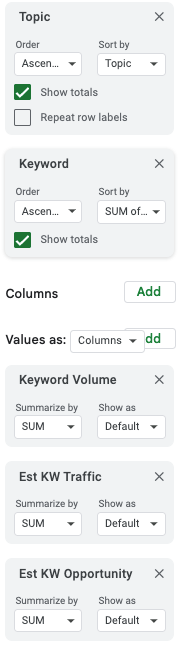
Add Topics, then Keywords below Topics. Then for values:
- Sum of Keyword Volume
- Sum of Est KW Traffic
- Sum of Est KW Opportunity
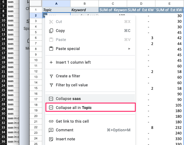
In Google Sheets, you can collapse all keywords into topics by right clicking on an open topic and then select “Collapse all in Topic”
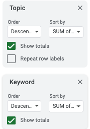
In Google Sheets, you can sort by using the righthand pivot table editor to choose:
- Sort Topic Descending by Sum of Est. Keyword Opportunity
- Sort Keyword Descending by Sum of Keyword Volume
This will give you topics prioritized by opportunity and within each topic, keywords will be listed by their volume.